Introduction
Physics simulation has been a well studied field in Computer Graphics. Recently, there has been efforts put in to do essentially the same task with deep learning. In our project, we looked at this paper. We replicated a navie version of their work and conducted experiments to learn GNN.
Tools and code we used
Follow the same setup as the paper, we used tensorflow 1, sonnet, graph_nets modules to build out network. We adapted the infrastructure such as dataloading, noise generation, and connectivity calculation directly from the original paper.
Dataset
We used the same dataset as the paper. It is generated by SPlisHSPlasH, a SPH-based fluid simulator.
Because we are both new to GNN, we focused more on the understanding other than the implementation side of this project. Experiments presented here are based on modification of the original code base. We also encountered difficulties with the speed of training and evaluation. So here we only present some preliminary results, which are enough to demonstrate substantial understanding of concepts.
Graph Neural Network
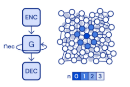
Graph neural network is a type of neural network that is based on graph structure. Information flows through the graph via message-passing between each node. To convert a problem into a graph, similar to what generally is done in language processing, we need to encode information first into a graph, then do message-passing steps, then decode the resulting state of the graph. Graph Neural network can easily captures spaitial information(e.g. distance between particles) or logical information(e.g. dependency in a computer program)
Our model structure
Input to our model is positions sequences of particles, with a length as a hyperparameter. The idea is to use the k-1 previous position to predict the current position k for each particle.
We preprocessed the data to do a high level feature extraction. We extracted: 1. the most important, connectivity of the graph through using a KDTree. 2. particles' distance to boundary the datset defines. Distance to 4 directions are calculated seperately. 3. distance between each nodes, in other words, weights on each edge in a graph. 4. velocity of each particle.
The encoder is responsible for encoding such high level features into a graph where later message-passing are preformed on. In every step of message-passing, information on each node is passed to its neighbors and with several message-passing steps, information is delivered further. Finally a decoder decodes the graph states. Same with the paper, we treat the decoded result as acceleration as we can use euler integration to calculate the next positon.
Notice that for encoder to encode a node, it uses multilayer perceptrons(MLP), a structure that is very similar to fully-connected layers, to encode node and edge features into a latent vectors. Decoder reverses this process.
Functionalities that were implemented in the paper are a superset of ours. It included more sophisticated features such as training noise, relative displacement. Our experiments were conducted on top of it
Experiments
What exactly is the network learning during training?
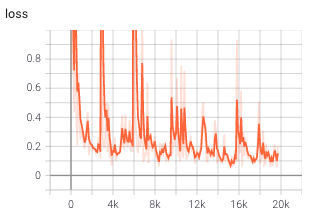
We used MSE loss during our training as we can easily apply it to accelerations. It is expected the model is going to produce larger error overtime during evalution because predictions are made based on preivous predictions. We were curious of when did the model start learning certain physical properties
 500 steps:

We can see the model already learned property of boundary. It also knows gravity. However, the attaction force seems to be over-represented in the model as clusters of particles are dragged up.
1000 steps:
Here we can see the boundary conditions are learned better as particles change direction on the upper boundary. Attraction force between particles are still too strong
2000 steps:
Notice that at step of 1000, particles experience a sudden acceleration to the left(we also see it later on), which didn't show up here. We suspect that there is a trend in the datset that when many particles are clustered together, there it is usually moving to the left. So through message passing, the whole clustered gained a leftward acceleration.
5000 steps:
Pretty much all phenomena observed previous were still here
10000 steps:
We were happy to see that gravity was learned universally. However, when particles were very close to each other, they exhibited no repelling force. Otherwise, they wouldn't statically state at the bottom when they first reached there
15000 steps:
Here the problem is more obvious. The physics engine that we used simulates an incompressible fluid. The model was incorrectly ignoring change in volume. But other than that it is very similar to the ground truth
20000 steps:
Lastly, some problems came back again. We found out that through out training, the model repetitively generating similar mistakes while learning a new feature, which proves the complexity of the problem. However, every time the mistakes were mitigated. At the last checkpoint, our model captures gravity, boundary, repulsion, and attractions. Through training more steps, the model will be able to produce higher quality result as the paper has demonstrated.
Tuning hyperparameters
Varying the number of message passing steps and evaluating performance
One of the unique features of a graph network is its ability for nodes to "talk" with one another via message passing. We seek to investigate the impact the distance messages can traverse on network performance and evaluate the importance of this parameter. Specifically we looked at four values for message passin: 3, 7, 10 (default) and 20. Note that the networks for 3 and 7 steps were both trained for 20,000 iterations. The networks for 10 and 20 steps were trained for 15,416 and 15985 iterations due to computational constraints. Additionally, the final smooth loss value was calculated using an exponential moving average with a weight of .5 .
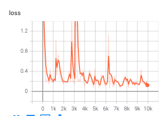
Step=3: Final Loss = .1550, Final Smoothed Loss = .1581
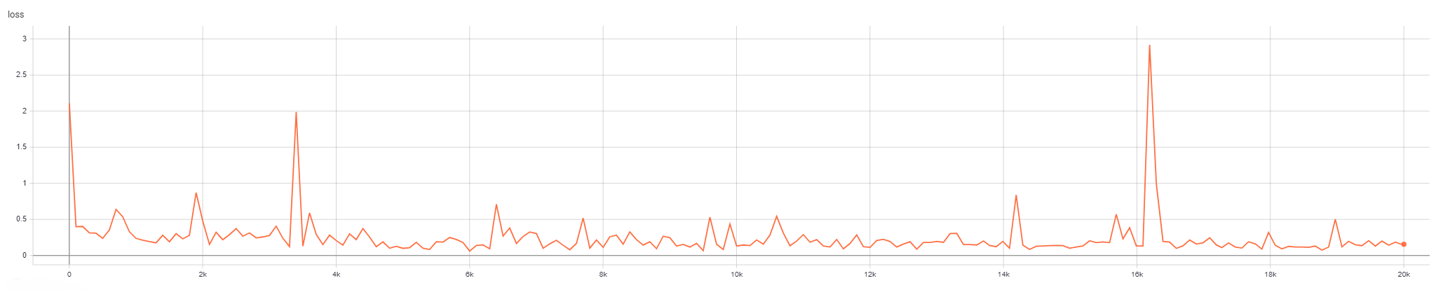
Step=7: Final Loss = .09631, Final Smoothed Loss = .1481
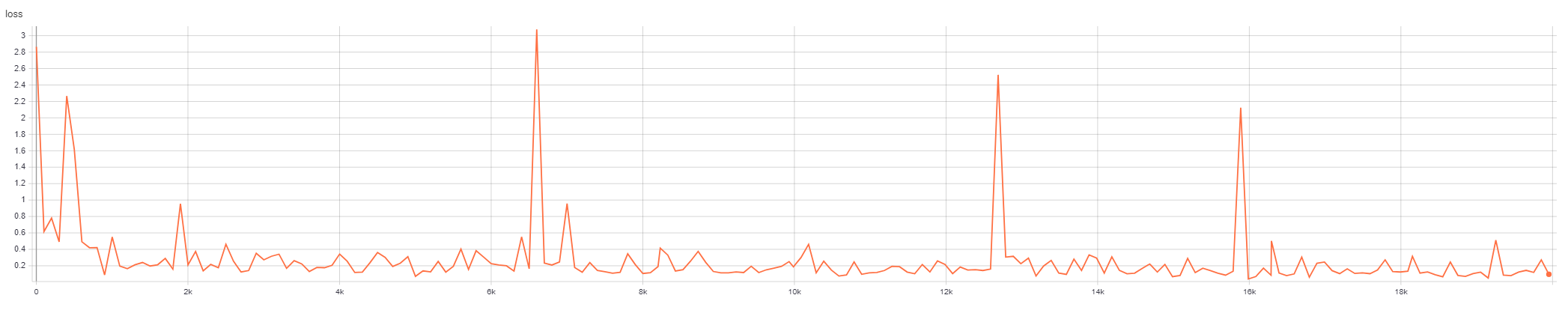
Step=10: Final Loss = .08881, Final Smoothed Loss = .1792
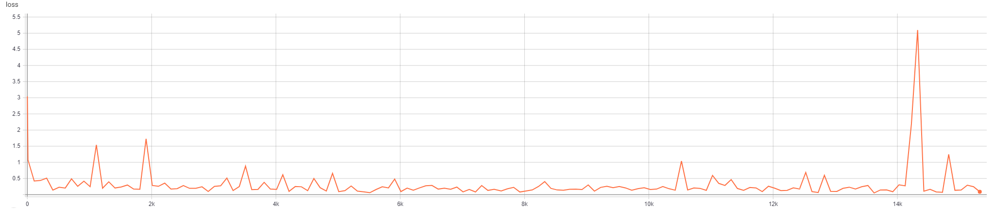
Step=20: Final Loss = .1637, Final Smoothed Loss = .1230
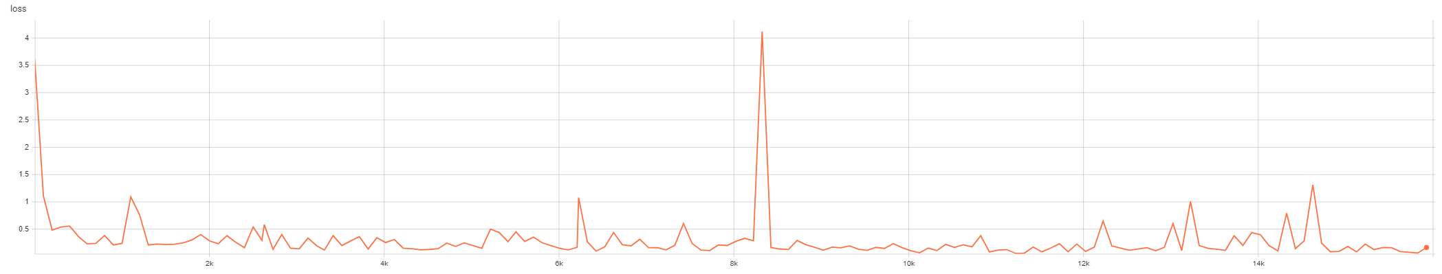
The model with 10 steps had the overal lowest final loss and the model with 20 steps had the overall lowest smoothed loss. There is no discernible difference regarding quality in terms of emulating the simulation. Each model performed relatively poorly on simulating the ground truth. This is in line with earlier results showing that even at 20000 iterations of training the models struggled to achieve high similarity with the ground truth. Due to computaitonal limitations, we were not able to train the models beyond this point; future work would center on training these models significantly longer to see if there is more of a discernible impact on the number of messaging steps.
Other Experiments
Changing the stride of residual connection in messeage-passing steps:
residual connection are implemented directly by adding the latent vectors of nodes and edges from a previous graph to the next graph. Previous residual connect is made every message step and we experiments. We experimented with adding stride to residual connection. We found that with larger residual step the training was smoother and the model was able to reach the loss as the original model. However, at 10000 steps, the model preforms bad as it didn't represent gravity well (it had similar behavior as the original network at 2000 steps).
Apply Layernorm for the decoder:
Previously Layernorm is applied in the encoding step and the message-passing steps. We apply layer normalization to the decoder. The last layernorm make the training more stable and the model converaged with a higher loss. This corresponds with what we learned in the class (for example, in CNN we don't apply batch normalization to the last step). We think that the last layer normalization will threshold important features that the graph generates. So the model was not able to learn much.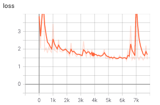
Different boundary conditions:
During feature extraction, the distance from particles to boundaries are normalized with the radius that also defines the connectivity. Then it was clip to -1 to 1. In previous experiments we found that particles were able to recognize boundaries but not very accurately. They behaves strangely when an acceleration drive them surpassing boundaries. Some started clusting, some even picked up another virtual boundary that was below the actual one. So we took away the clipping, hoping the model was able learn more by punish a larger negative value.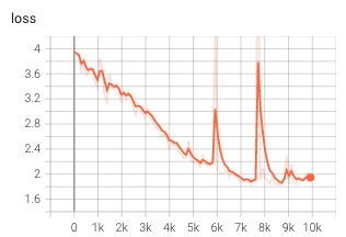 However, the training was very slow and the result animation does not show any physical property, so
we thought that this change confused the model.
However, the training was very slow and the result animation does not show any physical property, so
we thought that this change confused the model.